 |
 |
 |
Why Should You Use Nonlinear Curve Fitting?
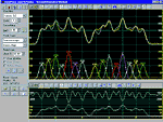
Nonlinear curve fitting is by far the most accurate way to reduce noise and quantify peaks. Many instruments come with software that only approximates the fitting process by simply integrating the raw data numerically. When there are shouldered or hidden peaks, a lot of noise or a significant background signal, this can lead to the wrong results. (For example, a spectroscopy data set may appear to have a peak with a 'raw' amplitude of 4,000 units -- but may have a shoulder peak that distorts the amplitude by 1,500 units! This would be a significant error.)
PeakFit helps you separate overlapping peaks by statistically fitting numerous peak functions to one data set, which can help you find even the most obscure patterns in your data. The background can be fit as a separate polynomial, exponential, logarithmic, hyperbolic or power model. This fitted baseline is then subtracted before peak characterization data (such as areas) is calculated, which gives much more accurate results. And any noise (like you get with electrophoretic gels or Raman spectra) that might bias raw data calculations is filtered simply by the nonlinear curve fitting process. Nonlinear curve fitting is essential for accurate peak analysis and accurate research.
PeakFit Offers Sophisticated Data Manipulation
|
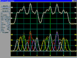
With PeakFit's visual FFT filter, you can inspect your data stream in the Fourier domain and zero higher frequency points -- and see your results immediately in the time-domain. This smoothing technique allows for superb noise reduction while maintaining the integrity of the original data stream. PeakFit also includes an automated FFT method as well as Gaussian convolution, the Savitzky-Golay method and the Loess algorithm for smoothing. AI Experts throughout the smoothing options and other parts of the program automatically help you to set many adjustments. And, PeakFit even has a digital data enhancer, which helps to analyze your sparse data. Only PeakFit offers so many different methods of data manipulation. |
|

Click to View Larger Image |
| |
Highly Advanced Baseline Subtraction
|
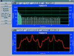
PeakFit's non-parametric baseline fitting routine easily removes the complex background of a DNA electrophoresis sample. PeakFit can also subtract eight other built-in baseline equations or it can subtract any baseline you've developed and stored in a file. |
|

Click to View Larger Image |
| |
| Full Graphical Placement of Peaks |
| |
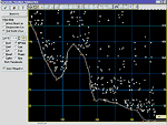
If PeakFit's auto-placement features fail on extremely complicated or noisy data, you can place and fit peaks graphically with only a few mouse clicks. Each placed function has "anchors" that adjust even the most highly complex functions, automatically changing that function's specific numeric parameters. PeakFit's graphical placement options handle even the most complex peaks as smoothly as Gaussians. |
| |
| Publication-Quality Graphs and Data Output |
| |
Every publication-quality graph (see above) was created using PeakFit's built-in graphic engine -- which now includes print preview and extensive file and clipboard export options. The numerical output is customizable so that you see only the content you want. |
| |
| PeakFit Saves You Precious Research Time |
| |
For most data sets, PeakFit does all the work for you. What once took hours now takes minutes – with only a few clicks of the mouse! It’s so easy that novices can learn how to use PeakFit in no time. And if you have extremely complex or noisy data sets, the sophistication and depth of PeakFit’s data manipulation techniques is unequaled. |
| |
| PeakFit Automatically Places Peaks in Three Ways |
| |
PeakFit uses three procedures to automatically place hidden peaks; while each is a strong solution, one method may work better with some data sets than the others.
-
The Residuals procedure initially places peaks by finding local maxima in a smoothed data stream. Hidden peaks are then optionally added where peaks in the residuals occur.
-
The Second Derivative procedure searches for local minima within a smoothed second derivative data stream. These local minima often reveal hidden peaks.
-
The Deconvolution procedure uses a Gaussian response function with a Fourier deconvolution/ filtering algorithm. A successfully deconvolved spec-trum will consist of “sharpened” peaks of equivalent area. The goal is to enhance the hidden peaks so that each represents a local maximum.
|
|

Click to View Larger Image

Click to View Larger Image
|